


How to Average Time in Excel?

If you’re looking to easily calculate average time in Excel, you’ve come to the right place. In this article, we’ll show you how to quickly and accurately calculate the average time in Excel by walking you through the process step by step. We’ll cover the basics of entering and formatting time values, as well as how to use some of the built-in functions in Excel for calculating average time. Ready to get started? Let’s jump right in!
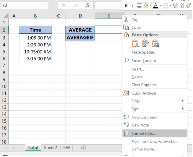
To average time in Excel, follow the steps below:
- Open the Excel spreadsheet containing the times you want to average.
- Press CTRL+SHIFT+: to enter the current time.
- Click on an empty cell and enter the formula =AVERAGE(.
- Click on the first cell containing the time you want to average and then drag your cursor to the last cell.
- Press ENTER to complete the formula.
- Press CTRL+ENTER to calculate the average time.
How to Use Excel to Calculate Time Averages
Excel is a powerful spreadsheet program that can be used to calculate averages for time periods. While the standard formula for calculating the average of a set of numbers is relatively straightforward, there are a few additional steps to take when dealing with time data. This guide will walk you through the process of calculating an average time in Excel.
Creating Time Data
Before you can calculate an average time in Excel, you will need to create a data set of time values. This can be done by entering the start and end times for each period into separate columns. Alternatively, you can create a single column containing the total time for each period.
Entering Time Values
When entering time values, it is important to make sure that the data is formatted correctly. Time values should be entered as a fraction of a day, such as 0.25 for 6 hours or 0.5 for 12 hours. This will ensure that the data is interpreted correctly by Excel.
Creating a Time Difference Column
If you have entered separate start and end times for each period, you will need to create a column containing the difference between the two. This can be done by subtracting the start time from the end time. Excel will automatically interpret the difference as a fraction of a day.
Calculating an Average Time
Once you have created a data set of time values, calculating an average time is fairly straightforward. To calculate the average time, simply use the AVERAGE function. This function will return the average of the time values in the specified range.
Formatting the Average Time Result
The AVERAGE function will return the average time as a fraction of a day. To view the result in a more readable format, you will need to format the cell containing the result. To do this, select the cell, click the “Number” tab in the “Format Cells” window, and select the “Time” category. This will display the average time in hours and minutes.
Using the Average Time Result
Once you have calculated and formatted the average time, you can use it in various ways. For instance, you can use it to calculate the average number of hours worked in a given period. You can also use it to compare the time spent on different tasks or to measure the efficiency of a particular process.
Conclusion
Calculating an average time in Excel is a relatively simple process. With the AVERAGE function and a few formatting adjustments, you can quickly and easily calculate an average time for any data set.
Few Frequently Asked Questions
Q1: How to calculate the average time in Excel?
A1: To calculate the average time in Excel, you need to first convert the time into the total number of minutes or seconds. To do this, you can use the formula =HOUR(cell)*60+MINUTE(cell). This will give you the total number of minutes or seconds for the time in that cell. You can then use the AVERAGE function to calculate the average of all the times. For example, if you have four cells with times in them, you can use the formula AVERAGE(cell1, cell2, cell3, cell4) to calculate the average time.
Q2: How to display the average time result in Excel?
A2: To display the average time result in Excel, you can use the TIME function. This function takes three arguments: the hour, minute, and second. To convert the average time result back into a time format, you can use the formula TIME(HOUR(AVERAGE(cell1, cell2, cell3, cell4)), MINUTE(AVERAGE(cell1, cell2, cell3, cell4)), SECOND(AVERAGE(cell1, cell2, cell3, cell4))). This will convert the average time result into a time format that can be displayed in Excel.
Q3: How to calculate the average of multiple time ranges in Excel?
A3: To calculate the average of multiple time ranges in Excel, you can use the AVERAGEIFS function. This function takes two arguments: the range of cells containing the time values, and the criteria of the time ranges that you want to average. For example, if you have a range of cells containing times in the format “HH:MM:SS”, and you want to average all the times that fall between 8:00 and 9:00, you can use the formula AVERAGEIFS(range, “>=8:00”, “Q4: How to calculate the average of multiple times with different units in Excel?
A4: To calculate the average of multiple times with different units in Excel, you can use the AVERAGEIFS function. This function takes three arguments: the range of cells containing the time values, the criteria of the time ranges that you want to average, and the unit of time that the values are in. For example, if you have a range of cells containing times in the format “HH:MM:SS”, and you want to average all the times that fall between 8:00 and 9:00, but some of the times are in minutes and some are in seconds, you can use the formula AVERAGEIFS(range, “>=8:00”, “Q5: How to calculate the average of multiple times based on multiple criteria in Excel?
A5: To calculate the average of multiple times based on multiple criteria in Excel, you can use the AVERAGEIFS function. This function takes four arguments: the range of cells containing the time values, the criteria of the time ranges that you want to average, the unit of time that the values are in, and the criteria of the additional data that you want to include in the average. For example, if you have a range of cells containing times in the format “HH:MM:SS”, and you want to average all the times that fall between 8:00 and 9:00, but you also want to include only times that are associated with a certain customer, you can use the formula AVERAGEIFS(range, “>=8:00”, “Q6: How to calculate the average of multiple times with different units and different criteria in Excel?
A6: To calculate the average of multiple times with different units and different criteria in Excel, you can use the AVERAGEIFS function. This function takes five arguments: the range of cells containing the time values, the criteria of the time ranges that you want to average, the unit of time that the values are in, the criteria of the additional data that you want to include in the average, and a logical operator that specifies how the criteria should be combined (i.e. “AND” or “OR”). For example, if you have a range of cells containing times in the format “HH:MM:SS”, and you want to average all the times that fall between 8:00 and 9:00, but you also want to include only times that are associated with a certain customer and a certain product, you can use the formula AVERAGEIFS(range, “>=8:00”, “