


How to Compare Two Excel Files for Duplicates?

Are you looking for an efficient way to compare two Excel files for duplicates? Look no further! In this article, you will discover a step-by-step guide on how to quickly and accurately compare two Excel files for duplicates. We will be covering topics such as using the VLOOKUP function, using Conditional Formatting, and using text comparison functions to make the task of identifying duplicates much easier. So, without further ado, let’s get started and learn how to compare two Excel files for duplicates.
Comparing two Excel files for duplicates can be done easily with Microsoft Excel’s “Conditional Formatting” tool. Follow these quick steps:
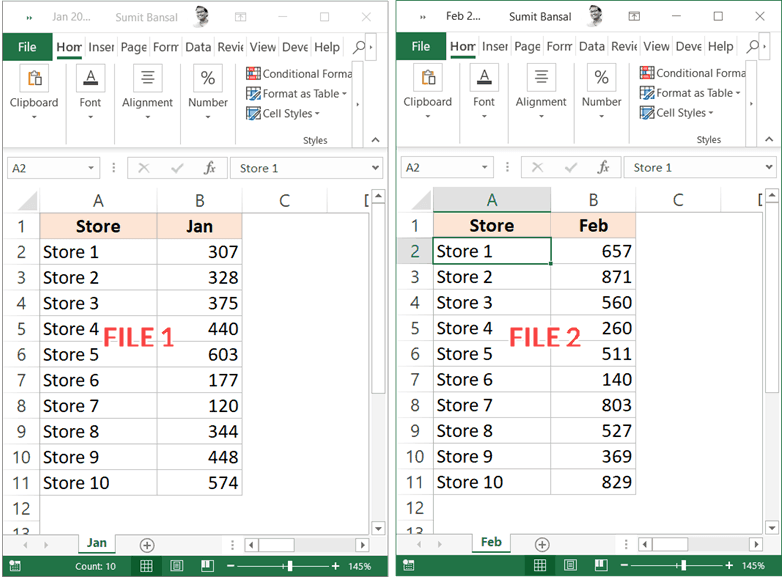
- Open both Excel files. Select the range of cells containing the data you want to compare.
- Go to Home tab, click on Conditional Formatting and then on “Highlight Duplicates”.
- The cells that are duplicates will be highlighted.
Using the ‘Conditional Formatting’ Feature to Compare Excel Sheets for Duplicates
Microsoft Excel offers a built-in feature called ‘Conditional Formatting’ that allows you to quickly and easily compare two Excel sheets for duplicates. This feature can be used to spot identical records across sheets, highlight cells that display the same values, and find and highlight unique records. In this article, we’ll explain how to use the Conditional Formatting feature to compare two Excel sheets for duplicates.
The Conditional Formatting feature works by applying a set of rules to a range of cells in an Excel sheet. When the conditions of the rules are met, the cells are highlighted according to the specified formatting. To compare two Excel sheets, you will need to create a ‘rule’ that specifies the conditions that must be met in order to highlight the cells as duplicates.
To begin, select the range of cells in the first Excel sheet that you want to compare. Then, select the ‘Conditional Formatting’ option from the ‘Home’ tab on the Ribbon. From the drop-down menu, select the ‘Highlight Cells Rules’ option. Next, select the ‘Duplicate Values’ option from the list of rules. This will open a dialog box where you can specify the formatting you would like to apply to the cells that meet the criteria of the ‘Duplicate Values’ rule.
Specifying the Duplicate Values Rule
Once you have opened the ‘Duplicate Values’ dialog box, you will need to select the cells in the second Excel sheet that you want to compare. To do this, click the ‘Choose another range’ option in the dialog box and select the range of cells in the second sheet. Once you have selected the range, you can specify the formatting you would like to apply to the cells that are identified as duplicates.
In the ‘Duplicate Values’ dialog box, you can select the color of the cell highlighting, the font style, and the font size. You can also specify if the highlighting should be applied to the entire row or just the cell that contains the duplicate values. When you have finished specifying the formatting, click the ‘OK’ button to apply the formatting to the cells that meet the criteria of the ‘Duplicate Values’ rule.
Testing the Duplicate Values Rule
Once you have applied the ‘Duplicate Values’ rule, you can test it to make sure that it is working correctly. To do this, you will need to enter some data into the cells in both Excel sheets that meet the criteria of the rule. For example, if you have specified that the rule should highlight cells that contain the same value, you should enter the same value into some of the cells in both sheets. Once you have entered the data, the cells should be highlighted according to the formatting you specified in the ‘Duplicate Values’ dialog box.
Using the Duplicate Values Rule to Compare Multiple Sheets
You can also use the ‘Duplicate Values’ rule to compare multiple Excel sheets. To do this, you will need to create a separate ‘Duplicate Values’ rule for each sheet you want to compare. You can then specify different formatting for each rule to make it easier to identify the duplicates in each sheet. Once you have created the rules, you can test them by entering some data into the cells in each sheet and verifying that the cells are highlighted correctly.
Removing the Duplicate Values Rule
If you no longer need the ‘Duplicate Values’ rule, you can remove it by selecting the range of cells that you applied the rule to and then selecting the ‘Conditional Formatting’ option from the ‘Home’ tab on the Ribbon. Next, select the ‘Clear Rules’ option from the drop-down menu. This will remove the ‘Duplicate Values’ rule and the formatting will be removed from the cells.
Related FAQ
What is the easiest way to compare two Excel files for duplicates?
The easiest way to compare two Excel files for duplicates is to use the “Remove Duplicates” feature. This feature is located in the Data tab of the ribbon, and it allows users to quickly compare two Excel files and eliminate duplicates. To use this feature, select the columns that you want to compare, then click the “Remove Duplicates” button. The feature will then scan the selected columns and delete any cells with duplicate data.
Can you compare two Excel files without the Remove Duplicates feature?
Yes, it is possible to compare two Excel files for duplicates without using the Remove Duplicates feature. One method is to use the VLOOKUP function. This function allows users to search for a value from one column in another column and return a value if it is found. To compare two Excel files, you can use the VLOOKUP function in one file to search for values in the other file, which will tell you if the values are duplicated.
What is the best way to compare two Excel files with a large number of rows?
The best way to compare two Excel files with a large number of rows is to use the Conditional Formatting feature. This feature can be found in the Home tab of the ribbon, and it allows users to quickly compare two columns of data and highlight any duplicates. To use this feature, select both columns, then click the “Conditional Formatting” button. Then select the “Duplicate Values” option, and the duplicates will be highlighted in both columns.
Can you compare two Excel files for differences instead of duplicates?
Yes, it is possible to compare two Excel files for differences instead of duplicates. One way to do this is to use the COUNTIFS function. This function allows users to compare two columns of data and count the number of cells with a matching value. To compare two Excel files for differences, you can use the COUNTIFS function in one file to search for values in the other file, which will tell you how many of the values are different.
What is the best way to compare two Excel files with a large number of columns?
The best way to compare two Excel files with a large number of columns is to use the Compare & Merge Workbooks feature. This feature is located in the Review tab of the ribbon, and it allows users to quickly compare two Excel files and highlight any differences. To use this feature, simply select both workbooks, then click the “Compare & Merge Workbooks” button. The feature will then scan both workbooks and highlight any differences.
What other methods are there for comparing two Excel files?
There are several other methods for comparing two Excel files. One method is to use the SUMIFS function. This function allows users to compare two columns of data and add up the values in one column where the values in the other column match. Another method is to use the IF function. This function allows users to compare two columns of data and return a value based on whether the values match or not. Finally, you can also use the FILTER function, which allows users to filter a range of cells based on specific criteria.
Excel – Conditional Formatting find duplicates on two worksheets by Chris Menard
Comparing two Excel files for duplicates is an important step in data management. By following the steps outlined in this article, you can quickly and easily identify any duplicates and ensure your data is organized and accurate. With the right tools and techniques, you can easily manage and compare your data, saving you time and effort in the long run.