


How to Freeze Both Row and Column in Excel?

Are you looking for ways to freeze both row and column in Excel? Excel is a powerful spreadsheet software from Microsoft and is widely used for creating and managing data. One of its powerful features is the ability to freeze both row and column in a worksheet. Freezing row and column helps you to work with large datasets efficiently, as it ensures that the top row and left-most column are always visible no matter how far down you scroll. In this article, we’ll take a look at how to freeze both row and column in Excel.
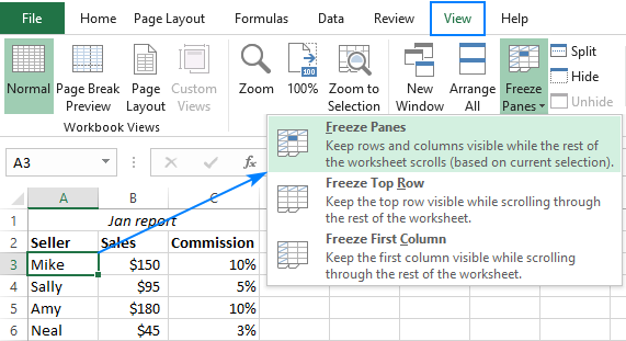
- Step 1: Select the cell below the rows and right of the columns you want to freeze.
- Step 2: Click the “View” tab and select “Freeze Panes.”
- Step 3: Click “Freeze Panes” and your rows and columns will be frozen.
Freezing Both Rows and Columns in Excel
Freezing row and column headings in an Excel worksheet can be a great help when you are working with a large amount of data. This feature allows you to keep the headings visible while scrolling through the rest of the worksheet. This article will explain how to freeze both rows and columns in an Excel worksheet.
Step 1: Select the Cell
The first step in freezing both rows and columns in an Excel worksheet is to select the cell that you want to be the starting point for your freeze. This should be the upper left-hand corner of the section of the worksheet that you want to keep visible. For example, if you wanted to freeze the first four rows and three columns, you would select cell A5.
Step 2: Freeze the Rows and Columns
Once you have selected the cell, you can then freeze the rows and columns. To do this, you will need to select the View tab on the Ribbon. Then, click the Freeze Panes drop-down menu and select either Freeze Top Row or Freeze First Column. This will freeze the rows and columns above and to the left of the selected cell.
Step 3: Unfreeze the Rows and Columns
If you ever need to unfreeze the rows and columns, you can do so by selecting the View tab on the Ribbon and then clicking on the Unfreeze Panes menu item. This will restore the worksheet to its original state.
Using Split Feature to Freeze Both Rows and Columns in Excel
The Split feature in Excel can be used to freeze both rows and columns in a worksheet. This feature allows you to divide the worksheet into multiple panes and then freeze the panes in place. To use this feature, you will need to select the View tab on the Ribbon and then click on the Split drop-down menu.
Step 1: Select the Area to Split
Once you have selected the Split drop-down menu, you will need to select the area of the worksheet that you want to split. This should be the area that you want to keep visible when you are scrolling through the worksheet. For example, if you wanted to freeze the first four rows and three columns, you would select cell A5.
Step 2: Split the Area
Once you have selected the area to split, you can then click on the Split button to divide the worksheet into multiple panes. You will then be able to scroll through each pane independently.
Step 3: Freeze the Panes
The last step is to freeze the panes in place. To do this, you will need to select the View tab on the Ribbon and then click on the Freeze Panes drop-down menu. This will freeze all of the panes in place so that the headings remain visible while you scroll through the worksheet.
Using the View Tab to Freeze Both Rows and Columns in Excel
The View tab in Excel can be used to freeze both rows and columns in an Excel worksheet. This feature allows you to keep the headings visible while scrolling through the rest of the worksheet. This article will explain how to use the View tab to freeze both rows and columns in an Excel worksheet.
Step 1: Select the View Tab
The first step in freezing both rows and columns in an Excel worksheet is to select the View tab on the Ribbon. This tab contains the Freeze Panes drop-down menu, which is used to freeze the rows and columns in place.
Step 2: Select the Cells to Freeze
Once you have selected the View tab, you will need to select the cells that you want to freeze. This should be the upper left-hand corner of the section of the worksheet that you want to keep visible. For example, if you wanted to freeze the first four rows and three columns, you would select cell A5.
Step 3: Freeze the Rows and Columns
Once you have selected the cells, you can then freeze the rows and columns. To do this, you will need to select the Freeze Panes drop-down menu and select either Freeze Top Row or Freeze First Column. This will freeze the rows and columns above and to the left of the selected cell.
Top 6 Frequently Asked Questions
Q1. What is meant by “Freezing” in Excel?
Ans: Freezing in Excel is the process of making certain rows or columns visible on the worksheet for the user, even when the user scrolls down or to the right. This allows the user to keep a reference to the information in the frozen rows or columns, while they work on the rest of the worksheet. This can be done by freezing both rows and columns.
Q2. How do I freeze both rows and columns in Excel?
Ans: To freeze both rows and columns in Excel, first select the row or column that you want to freeze. Then, open the View tab and select the Freeze Panes option. This will freeze the selected row or column, as well as all the rows and columns above and to the left of it.
Q3. How do I know if I have successfully frozen rows and columns in Excel?
Ans: You can tell that you have successfully frozen rows and columns in Excel if you notice a thick line running between the frozen row/column and the rest of the worksheet. Additionally, you may notice a different color for the row or column that is frozen.
Q4. Can I unfreeze the rows and columns once I have frozen them?
Ans: Yes, you can unfreeze the rows and columns once they are frozen. To do this, open the View tab and select the Unfreeze Panes option. This will unfreeze the rows and columns you had previously frozen.
Q5. Can I freeze multiple rows and columns at the same time?
Ans: Yes, you can freeze multiple rows and columns in Excel at the same time. To do this, select the rows and columns you want to freeze and then open the View tab and select the Freeze Panes option. This will freeze all of the selected rows and columns, as well as all the rows and columns above and to the left of them.
Q6. Is it possible to freeze only certain rows or columns?
Ans: Yes, it is possible to freeze only certain rows or columns in Excel. To do this, select the rows or columns you want to freeze and then open the View tab and select the Freeze Panes option. This will freeze the selected rows or columns, as well as all the rows and columns above and to the left of them.
How to freeze rows and columns at the same time in excel 2019
Learning how to freeze both row and column in Excel can save you a lot of time and frustration. With a few simple steps, you can easily manage your data and keep it organized. Freezing rows and columns in Excel can be a great way to keep track of your spreadsheet and allow quicker navigation and analysis of your data. So when you need to quickly navigate your spreadsheet, or you need to keep track of a specific row or column, freezing them can be a great way to do so.