How to Lookup Multiple Values in Excel?

Are you looking to make your Excel spreadsheet data more meaningful and organized? Excel is a powerful tool for data analysis and visualization, and one useful feature is the ability to look up multiple values in Excel. In this guide, you will learn how to use the LOOKUP function to find related values in a table or range of cells and use that information to make decisions or gain insights. You will also learn how to lookup multiple values using VLOOKUP and INDEX MATCH formulas. With these techniques, you’ll be able to quickly find the data you need in your Excel spreadsheets and make better decisions.

Using Excel to Lookup Multiple Values

Excel is a powerful tool that can be used to lookup multiple values quickly and efficiently. With its powerful features and functions, it can help you save time and make your work easier when it comes to looking up multiple values. In this article, we will discuss how to lookup multiple values in Excel and some of the best practices to make it easier.

Using VLOOKUP

One of the most common methods for looking up multiple values in Excel is to use the VLOOKUP function. This function will return the value of a cell based on the row and column numbers that you specify. For example, if you want to lookup the value in the third column of a table, you can use the VLOOKUP function to do so. This function is extremely versatile and can be used to lookup multiple values from different columns.

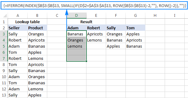
Using INDEX and MATCH

Another popular method for looking up multiple values in Excel is to use the INDEX and MATCH functions. This combination of functions can be used to look up multiple values from a single range of data. You can specify the row and column numbers that you want to look up, and the INDEX and MATCH functions will return the corresponding value from the range. This method is especially useful when you want to look up multiple values from a range that is larger than the number of columns you have in your table.

Using SUMIFS

The SUMIFS function is another powerful tool for looking up multiple values in Excel. This function allows you to specify multiple criteria for your lookup, and it will return the sum of all the values that meet your criteria. This makes it very useful for looking up multiple values from a larger range of data, such as a database table.

Using Pivot Tables

Pivot tables are an extremely powerful tool for looking up multiple values in Excel. A pivot table allows you to quickly summarize data from a larger range of data, and it can be used to look up multiple values quickly and easily. For example, you can use a pivot table to quickly look up the sum of sales for a particular product, or the average age of customers in a particular region.

Using Filters

Filters can be used to quickly and easily look up multiple values in Excel. You can specify the criteria for the filter, and Excel will automatically filter the data and return the values that meet your criteria. This makes it easy to quickly look up multiple values from a range of data.

Using Formulas

Formulas can also be used to look up multiple values in Excel. You can use formulas to quickly look up multiple values from a range of data, or to quickly calculate the sum or average of multiple values. For example, you can use a formula to quickly calculate the average age of customers in a particular region.

Using Macros

Macros can also be used to look up multiple values in Excel. Macros are small programs that can be used to automate tasks in Excel. You can use macros to quickly look up multiple values from a range of data, or to quickly calculate the sum or average of multiple values.

Using Conditional Formatting

One final method for looking up multiple values in Excel is to use conditional formatting. This feature allows you to quickly highlight cells that meet specific criteria. For example, you can quickly highlight cells that contain values greater than a certain number, or cells that contain text that meets a certain pattern. This makes it easy to quickly look up multiple values from a range of data.

Frequently Asked Questions

What is a Lookup Value in Excel?

A lookup value is a value that is used to search for a corresponding value in a data set. In Excel, lookup values can be used to find related information based on a single input. For example, if you have a list of employee names and corresponding employee numbers, you can use a lookup value to locate the employee number for a specific name.

What is the VLOOKUP Function?

The VLOOKUP function is a popular Excel function used to lookup and retrieve data from a specific column in a table. The VLOOKUP function takes a lookup value as an argument and searches for the value in the first column of the table array. Once the lookup value is found, the VLOOKUP function returns the corresponding value from another column in the table array.

How Do You Lookup Multiple Values in Excel?

To lookup multiple values in Excel, you can use the INDEX and MATCH functions together. The INDEX and MATCH functions allow you to search for multiple values in a data set and return corresponding data. To use the INDEX and MATCH functions, you must first create a lookup array that contains the lookup values you want to search for. Then, you can use the INDEX and MATCH functions to search for the lookup values in the lookup array and retrieve the corresponding values.

What is the Difference Between VLOOKUP and INDEX MATCH?

The main difference between VLOOKUP and INDEX MATCH is that VLOOKUP can only search for one value at a time, while INDEX MATCH can search for multiple values. VLOOKUP is also limited to searching in the first column of a table array. On the other hand, INDEX MATCH can search for values in any column of a table array. Additionally, INDEX MATCH can return multiple corresponding values from the same row, while VLOOKUP can only return a single result.

What is the Syntax for the INDEX and MATCH Functions?

The syntax for the INDEX and MATCH functions is as follows: INDEX(array, MATCH(lookup_value, lookup_array, 0)). The INDEX function requires an array argument, which is the range of cells containing the data you want to look up. The MATCH function requires three arguments: a lookup value, a lookup array, and a match type. The lookup value is the value you want to search for, the lookup array is the column containing the lookup values, and the match type is the type of match you want to perform (0 for exact match, 1 for approximate match).

What is the Limitation of the INDEX and MATCH Functions?

One of the main limitations of the INDEX and MATCH functions is that they cannot search for multiple lookup values in the same lookup array. To search for multiple values, you must use an array formula or a combination of other functions, such as the IF and OR functions. Additionally, the INDEX and MATCH functions cannot search for partial matches. To search for partial matches, you must use other functions, such as the SEARCH or FIND functions.

The power of Excel to look up multiple values can be an incredibly useful tool to have in your arsenal. By understanding how to use the various lookup functions, you can quickly and efficiently search through large amounts of data. With practice and experimentation, you can become an Excel expert and leverage the power of Excel to solve multiple problems quickly and accurately.