How to Shade Cells in Excel?

If you’re looking for a way to make your Excel spreadsheets stand out, shading cells is an easy and effective way to do it. With just a few clicks, you can make your data easier to read, distinguish important information, and make your spreadsheets look more professional. In this tutorial, we’ll show you how to shade cells in Excel, so you can start using this powerful tool to create visually appealing spreadsheets.

Shading cells in Excel is simple and easy. To shade a single cell, select the cell and click on the ‘Fill Color’ tool in the Home tab. You can also select multiple cells and shade them in one go by clicking on the Fill Color tool. To shade the entire row or column, select the row or column and click on the ‘Fill Color’ tool. You can also use the ‘Format Cells’ option to shade the cells based on their values.

Step 1: Select the cell or cells you would like to shade.
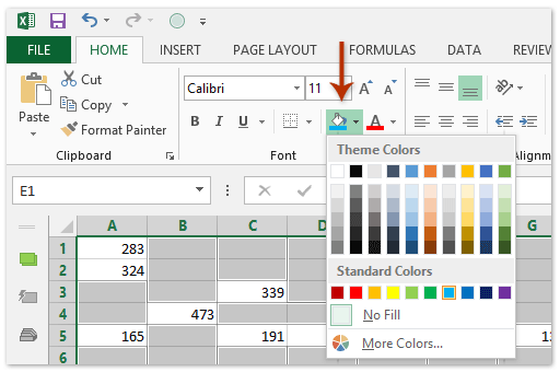
Step 2: Click on the ‘Fill Color’ tool in the Home tab.
Step 3: Choose a color from the color palette.
Step 4: To shade the entire row or column, select the row or column and click on the ‘Fill Color’ tool.
Step 5: Use the ‘Format Cells’ option to shade the cells based on their values.