


How To Use Roundup Function In Excel?

Are you looking for a comprehensive guide to understand and use the Roundup Function in Excel? This article will provide a detailed explanation of the Roundup Function and its uses, as well as a step-by-step tutorial on how to use it. To use the Roundup Function in Excel:
- Open the spreadsheet in Excel.
- Select the cell in which you want the result to be displayed.
- Type “=ROUNDUP(” in the selected cell.
- Enter the number or cell reference that you want to round.
- Enter the number of decimal places to which you want to round the number.
- Press Enter to get the result.
How Does Roundup Function Work In Excel?
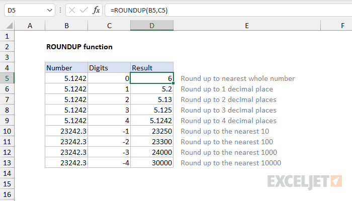
Roundup in Excel is a function that allows users to round numbers up to the nearest whole number, rounding up the decimal digits. This function can be used to quickly round up numbers in various applications, such as financial calculations and statistical analysis. To use the Roundup function in Excel, you must first select the cell or range of cells that you want to round up. Once you have selected the cell or range of cells, you can enter the formula “=ROUNDUP(Number,Decimals)” into the formula bar. The “Number” parameter is the number that you want to round up, and the “Decimals” parameter is the number of decimal places that you want to round up. After you have entered the formula, press enter to round up the number. The Roundup function in Excel will then round up the number to the nearest whole number, rounding up the decimal digits.
How Do You Round Up Data In Excel?
Rounding numbers in Excel is a quick and easy way to make your data easier to read and process. It is a useful tool for data analysis, and can be done with a few simple steps. To round up a number in Excel, the ROUNDUP function is used. This function takes two arguments: the number to be rounded and the number of digits to which the number should be rounded. For example, if we have a number with five digits, and we want to round it to two digits, we can use the formula =ROUNDUP(number, 2).
To use this function, first select the cell containing the number you want to round. Then, type in the formula, replacing “number” with the appropriate cell reference. For example, if the number is in cell A1, the formula would be =ROUNDUP(A1, 2). Then, press enter to calculate the result. This will round the number to two decimal places. You can also use the ROUNDUP function to round to a whole number, by setting the second argument to 0.
If you want to round a number up to the nearest 10, you can use the ROUNDUP function combined with the MROUND function. The MROUND function takes two arguments: the number to be rounded and the multiple to which it should be rounded. For example, if we want to round a number to the nearest 10, we can use the formula =MROUND(number, 10). To combine it with the ROUNDUP function, we can use the formula =ROUNDUP(MROUND(number, 10)). This will round the number up to the nearest 10. For example, if the number is 12.6, the result will be 20.
How Do You Use The Round Function In Excel With An Example?
The round function in Excel is a useful tool for quickly rounding numbers to a desired level of accuracy. This function can be used to round numbers up or down, depending on the user’s preferences. To use the round function in Excel, the user first needs to select the cells they wish to round. Next, they need to enter the formula “=ROUND(cell, number of decimal places).” The “cell” in the formula should be replaced with the cell containing the number to be rounded, and the “number of decimal places” should be replaced with the desired decimal place.
For example, if there is a cell containing the number 4.678, and the user wants to round it to the nearest tenth, they would enter =ROUND(4.678,1) into the formula bar. This formula would return the number 4.7, which is the nearest tenth of 4.678. Similarly, if the user wishes to round the number to the nearest hundredth, they would enter =ROUND(4.678,2) and the formula would return the number 4.68.
The round function in Excel can also be used to round numbers up or down, depending on the user’s preferences. To round a number up, the user needs to enter a negative number in the formula. For example, if the user wishes to round 4.678 up to the nearest tenth, they would need to enter =ROUND(4.678,-1). This formula would return the number 4.7. To round a number down, the user needs to enter a positive number in the formula. For example, if the user wishes to round 4.678 down to the nearest tenth, they would need to enter =ROUND(4.678,1). This formula would return the number 4.6.
The round function in Excel is a useful way to quickly round numbers to a desired level of accuracy. By entering the proper formula into the formula bar, the user can easily round numbers up or down, depending on their preferences.
How Do You Enter A Formula Using The Roundup And Average Function In Excel?
Entering a formula using the roundup and average functions in Excel is fairly straightforward. To begin, open up Excel and select the cell in which you would like to enter the formula. Click the “Formulas” tab and select “More Functions” from the drop-down list. From the “Select a function” list, select the “ROUNDUP” function. This will bring up a dialog box with the syntax for the roundup formula.
The syntax for the Roundup function is “ROUNDUP(number, num_digits)”. In this syntax, the number refers to the value that you would like to round up, and the num_digits refers to the number of decimal places that you would like the value to be rounded up to. For example, if you enter “ROUNDUP(2.55, 0)” into a cell, the value of that cell will be rounded up to 3. Next, select the “AVERAGE” function from the “Select a function” list. This will bring up a dialog box with the syntax for the average formula.
The syntax for the Average function is “AVERAGE(number1,
Excel Round Up To Nearest Whole Number
The Roundup function in Excel is a powerful tool for rounding numbers to the nearest whole number. It is an incredibly useful function to have when working with large numbers or fractions, as it can quickly and easily round numbers up or down. In this tutorial, we will show you how to use the Roundup function in Excel.
To use the Roundup function in Excel, first, open a spreadsheet and select the cell where you want to enter the Roundup formula. Then, type in the formula “=ROUNDUP(number, number of digits)” where number is the number you want to round up and number of digits is the number of digits you want to round to. For example, if you want to round the number 4.5 up to the nearest whole number, the formula would be “=ROUNDUP(4.5,0)”. The result of this formula will be 5.
You can also use the Roundup function to round down a number to the nearest whole number. To do this, type the formula “=ROUNDDOWN(number, number of digits)” in the cell where you want to enter the formula. For example, if you want to round the number 4.5 down to the nearest whole number, the formula would be “=ROUNDDOWN(4.5,0)” and the result of this formula will be 4.
Using the Roundup function in Excel is a great way to quickly and easily round numbers to the nearest whole number. With this function, you can easily round up or down any number without having to manually calculate the result.
Excel Round Up To Nearest 100
The Roundup Function in Excel is a useful tool for rounding numerical values up to the nearest specified multiple. It is useful when dealing with large numbers of figures, as it reduces the amount of time needed to calculate the nearest multiple manually.
To use the Roundup Function in Excel, follow these steps:
- Open your Excel spreadsheet and select the cell(s) containing the number(s) you want to round up.
- Click on “Formulas” and select “Math & Trig” from the drop-down menu.
- Select “Roundup” from the list of functions.
- Enter the multiple you want to round up to in the “Number” box.
- Enter the numerical value you want to round up in the “Significance” box.
- Click “OK” to calculate the result.
The result of the Roundup Function will be the nearest multiple of the number you entered in the “Number” box. For example, if you entered 100 in the “Number” box and 123 in the “Significance” box, the result will be 200.
Roundup Formula
The Roundup function in Excel is a mathematical function that rounds a number up to a specified multiple. This function is useful when dealing with large data sets, as it helps to reduce the amount of work required to round up numbers. To use the roundup function, the syntax is:
ROUNDUP (number, multiple).
The number argument is the number that you want to round up, and the multiple argument is the multiple that you want the number to be rounded up to. For example, if the number is 4.3 and the multiple is 0.5, then the result would be 4.5.
The roundup function is also useful when dealing with decimal numbers. For example, if the number is 4.75 and the multiple is 0.25, then the result would be 5.0. The roundup function can also be used to round up numbers to the nearest integer. For example, if the number is 4.7 and the multiple is 1, then the result would be 5.
In conclusion, the Roundup function in Excel is a useful mathematical function that can help you to quickly round up numbers to a specified multiple. This can be helpful when dealing with large data sets, or when dealing with decimal numbers.
How To Round Up Decimals In Excel
The Roundup function in Excel is a great way to quickly round up decimals to the nearest whole number. This is especially useful for financial calculations, such as when calculating taxes or interest. To use the Roundup function in Excel, you will need to first open the spreadsheet on which you wish to perform the calculation.
Once the spreadsheet is open, you will need to select the cell in which you want to display your rounded-up value. Then, type the formula =ROUNDUP(number, num_digits) into the cell. The number in the formula is the decimal or real number you want to round up. The num_digits is the number of digits to which you want to round up the number. For example, if you want to round up a decimal number to the nearest whole number, you need to set num_digits to 0.
Once you have entered the formula, press enter to execute the formula and the result will be displayed in the cell. The result will be the number rounded up to the nearest whole number, according to the num_digits parameter you have set. For example, if you have a decimal number of 3.14 and you set num_digits to 0, the result will be 4.
The Roundup function in Excel is a great way to quickly round up decimals to the nearest whole number. This can save time and be useful for financial calculations. To use the Roundup function, you will need to open the spreadsheet and enter the formula =ROUNDUP(number, num_digits) into the cell. Then, press enter to execute the formula and the result will be the number rounded up to the nearest whole number, according to the num_digits parameter you have set.
Excel Round Up To Nearest 5
The Roundup function in Excel is a powerful tool that can be used to round numbers up to the nearest integer. It is particularly useful for financial calculations, such as calculating the amount of interest earned on a loan or the amount of tax due on an income. This article will explain how to use the Roundup function in Excel.
To use the Roundup function in Excel, you must first select the cell in which you would like the result to appear. Then, enter the formula =ROUNDUP(number,num_digits) into the cell. The number is the value you would like to round up, and num_digits is the number of decimal places to which you would like to round up the number. For instance, if you would like to round up the value 10.5 to the nearest integer, you would enter the formula =ROUNDUP(10.5,0).
The Roundup function can also be used to round up a range of numbers. To do this, enter the formula =ROUNDUP(number,num_digits) into the first cell of the range. Then, drag the formula down to the last cell of the range. This will apply the Roundup formula to all of the cells in the range.
The Roundup function in Excel is a powerful tool that can make rounding numbers up to the nearest integer a breeze. With just a few simple steps, you can use the Roundup function to quickly and accurately round up any number or range of numbers in Excel.
Mround Function In Excel
The MROUND Function in Excel is a statistical function that allows you to round a number to the nearest multiple of another number. This function is useful for rounding to a specific increment, such as rounding a number to the nearest ten, hundred, or even thousand. It is also useful for finding the nearest multiple of a number.
To use the MROUND function, you must enter two arguments – the number you want to round and the multiple you want to round to. The function will then return the nearest multiple of the second argument. For example, if you enter the number 5.5 and the multiple of 3, the MROUND function will return 6.
The MROUND function is especially useful for creating formulas in Excel that require specific increments. For example, if you are creating a formula to calculate a sales tax, you could use the MROUND function to ensure that the result is rounded to the nearest cent. You could also use the MROUND function to round a number to the nearest multiple of 10, such as rounding a number to the nearest 10, 100, or even 1000.
The MROUND function is a great tool for rounding numbers to specific multiples and is easy to use with just two arguments. It is a great way to ensure that your calculations are accurate and to ensure that your results are rounded to the nearest multiple.
Excel Round Up To Nearest 1000
The Roundup function in Excel is a mathematical function that allows you to round a number up to a specified multiple. This function can be used to round a number to the nearest 1000, 10,000, 100,000, and so on. To use the Roundup function in Excel, you need to enter a formula in the desired cell and specify the number to round and the multiple to round it up to.
To use the Roundup function in Excel, you need to enter the formula =ROUNDUP(number,multiple) in the desired cell. The “number” is the number you want to round up and the “multiple” is the multiple you want to round the number up to. For example, if you want to round up the number 8,456 to the nearest 1,000, you would enter the formula =ROUNDUP(8456,1000). This will round 8,456 up to 9,000.
To round up a number to the nearest 1,000, you need to enter the formula =ROUNDUP(number,1000) in the desired cell. The “number” is the number you want to round up and the “multiple” is set to 1000. For example, if you want to round up the number 8,456 to the nearest 1,000, you would enter the formula =ROUNDUP(8456,1000). This will round 8,456 up to 9,000.
You can also use the Roundup function in Excel to round numbers up to the nearest 10, 100, 10,000, and so on. To do this, you will need to modify the formula to =ROUNDUP(number,multiple). For example, if you want to round up the number 8,456 to the nearest 10, you would enter the formula =ROUNDUP(8456,10). This will round 8,456 up to 8460.
Excel Roundup(sum)
The Roundup function in Excel is a useful tool for rounding up a number to a desired precision. It is a built-in Excel function that can be used to round up a number to the nearest multiple of a given number. Roundup is also referred to as the Round-Up function and is available in both Microsoft Excel and LibreOffice Calc.
To use the Roundup function in Excel:
- Open the Excel spreadsheet you wish to use.
- In the cell where you want the result of the Roundup function to appear, type =roundup(sum).
- Replace “sum” with the cell reference of the number you wish to round up.
- Type in the multiple you wish to round up the number to, inside the parentheses after the “sum”.
- Press Enter to apply the Roundup function.
The Roundup function in Excel is a convenient and easy way to quickly round up a number to the nearest multiple of your choice. This can be useful for various calculations such as calculating discounts, taxes, or other financial operations.
How to ROUNDUP in Excel
In conclusion, learning how to use the Roundup function in Excel is a great way to quickly and easily round numbers up or down. It can save time and makes it easier to work with large amounts of data. With a few simple steps, you can use this useful tool to help you become more efficient and productive in your day to day work.