How to Use the Roundup Function in Excel?

If you’ve ever found yourself in a situation where you need to quickly summarize a large amount of data in Excel, then the Roundup function is your go-to solution. This helpful Excel feature can help you quickly and easily perform calculations on your data, saving you time and effort while giving you accurate results. In this article, we’ll break down how to use the Roundup function in Excel and explain why it is such a useful tool. So, let’s get started!

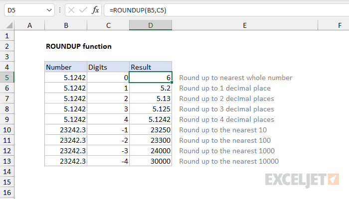
The Roundup function in Excel is a great way to quickly round numbers up to a specific multiple. To use the function:

Go to the cell where you would like to enter the rounded-up number.
Enter the formula “=ROUNDUP(number, num_digits)”.
Replace “number” with the number you would like to round up, and “num_digits” with the multiple you would like to round to (e.g. 0.5, 1, 5, 10, etc.).
Press enter to get your rounded-up result.

What is the Roundup Function in Excel?

The Roundup Function in Excel is a mathematical function that rounds a number up to the nearest specified digit. For example, if you enter 2.3 into the function, it will round the number up to 3. This function is useful for quickly adjusting decimal places, setting currency amounts to the nearest whole number, and for making calculations easier for those who are new to Excel.

The Roundup Function in Excel is part of the Microsoft Office suite and is available in all versions of Excel since 2007. It is easy to use and can be accessed from the “Formulas” menu in Excel. This function is also available in other spreadsheet programs such as Google Sheets and Apple Numbers.

How to Use the Roundup Function in Excel?

Step 1: Enter the Number to be Rounded Up

The first step in using the Roundup Function in Excel is to enter the number that you want to round up. This can be done in any cell within the spreadsheet. Simply type the number into the cell and press “Enter”.

Step 2: Select the Roundup Function

Once you have entered the number, you can select the Roundup Function from the “Formulas” menu. This will open a dialog box where you can select the number of digits you want to round up to. You can choose from 1 to 9 digits, or you can specify a custom number of digits.

Step 3: Enter the Cell of the Number to be Rounded Up

The next step is to enter the cell that contains the number you want to round up. This can be done by clicking on the cell and then clicking “OK” in the dialog box. This will insert the Roundup Function into the cell.

Tips for Using the Roundup Function in Excel

Tip 1: Use the Rounddown Function for Numbers Below the Specified Digit

The Roundup Function in Excel is designed to round up numbers to the nearest specified digit. If you want to round down numbers that are below the specified digit, you can use the Rounddown Function. This can be accessed from the “Formulas” menu in Excel.

Tip 2: Use the Round Function for Whole Numbers

The Roundup Function in Excel can be used to round up numbers to the nearest specified digit. However, if you want to round a number to the nearest whole number, you can use the Round Function. This can be accessed from the “Formulas” menu in Excel.

Troubleshooting the Roundup Function in Excel

Problem 1: Not Getting the Desired Result

If you are not getting the desired result when using the Roundup Function in Excel, make sure that you have entered the correct cell for the number to be rounded up. Also, make sure that you have selected the correct number of digits to round up to.

Problem 2: Not Finding the Roundup Function in Excel

If you are having trouble finding the Roundup Function in Excel, make sure that you are in the “Formulas” menu. This is the menu where the Roundup Function can be found. If you are still having trouble, you can search for the function in the “Help” menu.