


How to Do Linest in Excel?

Are you an Excel user looking to learn how to draw lines on your worksheets? Drawing lines in Excel is a great way to add visual clarity and emphasis to your spreadsheets. In this article, we’ll take a look at the various ways you can draw lines in Excel, from simple borders to complex shapes. Plus, we’ll provide helpful tips and tricks for creating the perfect lines for your spreadsheets. Let’s get started!
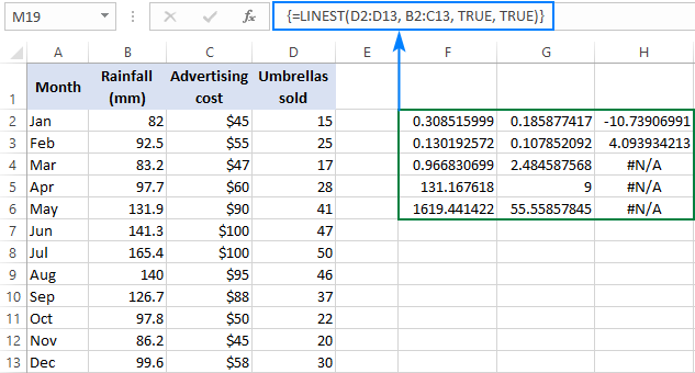
Linest in Excel is a statistical function used to calculate and create a least-squares regression line from the data points in a table. To use the function, select the range of cells containing the data points, then enter the LINEST function into the formula bar. The function will calculate the parameters of the line and provide the equation of the line as output. To improve accuracy, it is recommended to enter the known x-values into the last column of the data range and the known y-values into the first column of the data range.
- Open the Excel spreadsheet with the data points.
- Select the range of cells containing the data points.
- Enter the LINEST function into the formula bar.
- Enter the known x-values into the last column of the data range.
- Enter the known y-values into the first column of the data range.
- Press Enter to calculate the parameters of the line.
What is a Line of Best Fit in Excel?
A line of best fit is a line that best represents the data points of a chart in Microsoft Excel. It is used to predict outcomes and to analyze trends in a dataset. The line is created by finding the equation of a straight line that minimizes the sum of the squared residuals, which are the distances between the data points and the line. The line of best fit is used to determine the relationship between two or more variables and can be used to make predictions about future data points.
The equation of the line of best fit is typically used to calculate the slope and intercept of the line. The slope of the line can be used to calculate the rate of change between the two data points and the intercept of the line can be used to calculate the point at which the line crosses the y-axis.
How to Create a Line of Best Fit in Excel
Creating a line of best fit in Excel is a relatively straightforward process. The first step is to create a chart and add the data points to the chart. The data points can be added either by manually entering the data points or by importing the data from another source. Once the data points have been added, it is time to add the line of best fit.
The next step is to click on the “Layout” tab, which can be found in the top ribbon of the chart. Once the Layout tab is selected, click on the “Trendline” option and then select the type of line of best fit you would like to use. The most commonly used line of best fit is the “Linear” option, but other options such as “Polynomial” and “Exponential” are also available.
Once the type of line of best fit has been selected, the equation of the line of best fit will be displayed in the chart. This equation can be used to calculate the slope and intercept of the line.
How to Use the Line of Best Fit
Once the line of best fit has been created, it can be used for a variety of purposes. The most common use is to make predictions about future data points. The equation of the line can be used to calculate the rate of change between two data points and the intercept of the line can be used to calculate the point at which the line crosses the y-axis.
In addition to predicting future data points, the line of best fit can also be used to analyze trends in a dataset. The slope of the line can be used to determine the rate of change between the two data points and the intercept of the line can be used to calculate the point at which the line crosses the y-axis. This can be used to determine if there is a linear or non-linear relationship between the two data points.
How to Modify the Line of Best Fit in Excel
Once the line of best fit has been created, it can be modified in a variety of ways. The first step is to click on the “Layout” tab, which is located in the top ribbon of the chart. Once the Layout tab is selected, click on the “Trendline” option and then select the “Format Trendline” option.
From the Format Trendline menu, users can select different options such as the line color, line width, and line style. Additionally, users can also select the “Options” tab, which will allow users to modify the equation of the line of best fit. This includes modifying the intercept, slope, and coefficient values of the equation.
How to Add a Second Line of Best Fit in Excel
It is also possible to add a second line of best fit to an existing chart. To do this, click on the “Layout” tab and then select the “Trendline” option. Once the Trendline option is selected, click on the “More Trendline Options” option.
From the More Trendline Options menu, users can select the “Add Trendline” option to add a second line of best fit to the existing chart. This line can be customized in the same way as the original line of best fit. Additionally, users can add additional lines of best fit by repeating the same steps.
Frequently Asked Questions
What is a Line Graph in Excel?
A line graph in Excel is a chart type that shows trends over time or breaks down changes in data over a set period. This type of graph is very useful for visualizing changes in data over time, or for comparing different entities with each other. It is one of the most popular chart types used in Excel and is easy to create. Line graphs can be used to show trends over time, such as the growth of a company’s sales or the changes in the stock market. They can also be used to compare different entities, such as the sales of different products or the performance of different teams. Line graphs can help to identify patterns in data and can be used to make predictions about future trends.
How do I create a line graph in Excel?
Creating a line graph in Excel is very easy. Start by opening a new workbook and entering your data into the spreadsheet. Then, select the data you want to include in your graph. To create the line graph, go to the Insert tab and select the Line chart option. You can then choose the type of line graph you want to create, such as a simple line graph or a scatter plot. Once you have chosen the type of graph, click Insert to create the graph. You can then customize the graph by changing its colors, adding labels, and adding a title.
What are the advantages of using Line Graphs?
Line graphs are a great way to visualize changes in data over time or to compare different entities. Line graphs can help identify patterns and trends in data that may not be apparent in other types of charts. They are also easy to create and customize, making them a great choice for visualizing data. Line graphs can also help to make predictions about future trends.
What are the different types of Line Graphs?
There are several different types of line graphs that can be used in Excel. The most common are simple line graphs, which are used to show trends over time, such as the growth of a company’s sales. Scatter plots are used to compare different entities, such as the sales of different products or the performance of different teams. Step graphs are used to show changes in discrete units of time, such as months or years. Finally, area graphs are used to show the overall trend of a set of data points.
What are the best practices for creating Line Graphs?
When creating line graphs, it is important to make sure that the data is accurate and up-to-date. Additionally, it is important to make sure that the graph is easy to read and understand. The labels and titles should be clear and descriptive, and the colors should be chosen carefully so that they are easy to distinguish. Finally, it is important to ensure that the graph is not cluttered with too much information.
What are some tips for making Line Graphs more effective?
When creating line graphs, it is important to use the right type of graph for the data being presented. Additionally, it is important to make sure that the graph is easy to read and understand. The labels and titles should be clear and descriptive, and the colors should be chosen carefully so that they are easy to distinguish. Finally, it is important to use the right scale for the data being presented. This will ensure that the graph is accurate and that the changes in data can be seen clearly. Additionally, it is important to make sure that the graph is not cluttered with too much information.
The bottom line is that knowing how to do lines in Excel is a great skill to have. It can help you create tables, charts, and other visuals to help you organize and present your data. With a little practice, you can become an expert in creating lines in Excel, and you’ll be ready to take on any task that requires this skill.