How to Highlight Cells in Excel Based on Text?

Are you looking for a quick and easy way to highlight cells in Excel based on text? Look no further! In this article, we’ll walk you through the simple steps for highlighting cells in Excel that contain specific text. We’ll provide helpful tips and tricks for customizing your highlights, so you can make the information in your spreadsheets stand out. Let’s get started!

Highlighting cells in Excel based on text is a simple process. To get started, open the Excel file you want to work with. Select the cells you want to highlight, click the Conditional Formatting button on the Home tab, and then select Highlight Cell Rules. Choose Text that Contains, and enter the text you want to highlight. Then, choose the formatting you want to apply. Finally, click OK to apply.

Alternatively, if you want to compare two or more text terms within a cell, you can use the Highlight Cell Rules option to create a comparison table. Select the cells you want to compare and click the Conditional Formatting button on the Home tab. Then, select Highlight Cell Rules and choose Text that Contains. Enter the text you want to compare in the rule criteria box and select the formatting to apply for each term. Finally, click OK to apply the comparison table.

Highlighting Cells in Excel Based on Text

Highlighting cells in Excel based on text is a great way to quickly identify values in a range. This technique can be used to find errors, highlight key information, or just to make a worksheet easier to read. In this article, we will discuss how to highlight cells in Excel based on text.

Using the Conditional Formatting Feature

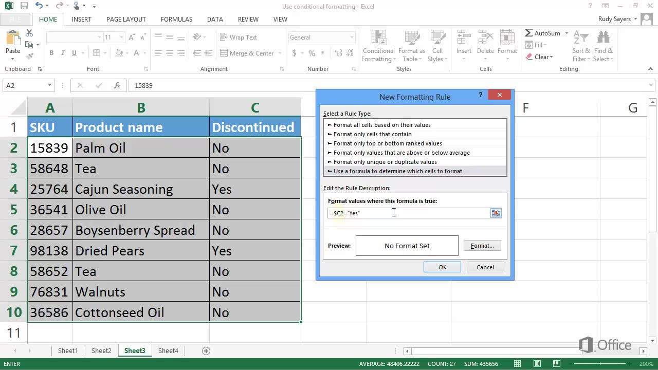
The easiest way to highlight cells in Excel based on text is to use the Conditional Formatting feature. This feature allows you to set up rules that will automatically apply formats to cells based on certain conditions. To use this feature, select the range of cells you want to format and then click on the Home tab. In the Styles group, click on Conditional Formatting and then select New Rule.

In the New Formatting Rule window, select Use a formula to determine which cells to format. In the Format values where this formula is true box, enter the formula you want to use. For example, if you want to highlight cells containing the word “error”, the formula would be =$A1=”error”. Click Format and then select the formatting you want to apply to the cells. Finally, click OK to apply the rule.

Using the Find and Replace Feature

Another way to highlight cells in Excel based on text is to use the Find and Replace feature. This feature allows you to quickly search for specific text and then replace it with another value. To use this feature, select the range of cells you want to search and then click on the Home tab. In the Editing group, click on Find & Select and then select Find.

In the Find and Replace window, enter the text you want to search for in the Find what box. In the Replace with box, enter the formatting you want to apply to the cells. For example, if you want to highlight cells containing the word “error”, you would enter the formatting in the Replace with box. Click Find Next to search for the text and then click Replace to apply the formatting.

Using the Filter Feature

The final way to highlight cells in Excel based on text is to use the Filter feature. This feature allows you to filter a range of cells based on specific criteria. To use this feature, select the range of cells you want to filter and then click on the Data tab. In the Sort & Filter group, click on Filter.

In the Filter window, select the column you want to filter and then select Text Filters. In the drop-down menu, select Contains. In the box next to Contains, enter the text you want to filter for. For example, if you want to highlight cells containing the word “error”, you would enter “error” in the box. Click OK to apply the filter.

Using the IF Function

The IF function in Excel can also be used to highlight cells based on text. This function allows you to set up rules that will return a value if the criteria are met. To use this function, enter the formula =IF($A1=”error”, “Highlight”, “”) in the cell where you want to apply the formatting. This formula will check the cell for the text “error” and if it is found, the cell will be highlighted.

Using the COUNTIF Function

The COUNTIF function in Excel can also be used to highlight cells based on text. This function allows you to count the number of cells in a range containing a certain value. To use this function, enter the formula =COUNTIF($A1:$A10,”error”) in the cell where you want to apply the formatting. This formula will count the number of cells in the range containing the text “error” and if it is found, the cell will be highlighted.

Using the VLOOKUP Function

The VLOOKUP function in Excel can also be used to highlight cells based on text. This function allows you to search for a specific value in a range. To use this function, enter the formula =VLOOKUP($A1,”Error List”,1,FALSE) in the cell where you want to apply the formatting. This formula will search for the text “error” in the range “Error List” and if it is found, the cell will be highlighted.

Using the SUMIF Function

The SUMIF function in Excel can also be used to highlight cells based on text. This function allows you to sum a range of cells based on a certain criteria. To use this function, enter the formula =SUMIF($A1:$A10,”error”,$B1:$B10) in the cell where you want to apply the formatting. This formula will sum the values in the range “B1:B10” if the text “error” is found in the range “A1:A10” and if it is found, the cell will be highlighted.

Frequently Asked Questions

What is Cell Highlighting in Excel?

Cell highlighting in Excel is a feature that allows the user to highlight specific cells based on the contents of the cell. This can be done through the use of conditional formatting, which allows the user to specify criteria for a cell to be highlighted, such as when the cell contains a certain text string. This feature can be useful for quickly identifying cells that contain specific information.

What is the Process for Highlighting Cells in Excel Based on Text?

The process for highlighting cells in Excel based on text is relatively simple and straightforward. First, the user must select the cells they wish to highlight. Then, the user must click on the Home tab and select Conditional Formatting from the Styles group. Here, the user can select New Rule and then select Format only cells that contain from the list of options. The user can then enter the text they wish to highlight and select the desired formatting. Finally, the user can click OK and the specified cells will be highlighted accordingly.

What are Some Examples of Commonly Used Highlighting Rules?

Some examples of commonly used highlighting rules include highlighting cells that contain specific text, such as a name or an address; highlighting cells that contain specific numbers, such as an amount or a percentage; and highlighting cells that are greater than or less than a certain value. Additionally, users can also create rules that highlight cells based on more complex criteria, such as cells that contain a specific text string and a specific number.

What are the Benefits of Highlighting Cells in Excel Based on Text?

The primary benefit of highlighting cells in Excel based on text is that it can make it easier to identify specific cells and data points within a spreadsheet. This can be particularly useful for larger spreadsheets, as it makes it easier to quickly identify cells that are relevant to a particular task. Additionally, this feature can make it easier to apply formatting to specific cells, such as changing the font color or adding a background color.

Are there Any Limitations to Highlighting Cells in Excel Based on Text?

Yes, there are some limitations to highlighting cells in Excel based on text. For example, cells can only be highlighted based on the contents of the cell and not based on the value of the cell. Additionally, this feature can only be used to highlight cells, and cannot be used to apply other formatting options such as changing the font color or adding a background color.

How Do I Change the Highlighting Settings for Cells in Excel?

The highlighting settings for cells in Excel can be changed by selecting the cells and then clicking on the Home tab and selecting Conditional Formatting from the Styles group. Here, the user can select Edit Rule and then make changes to the criteria for highlighting the cells. Additionally, the user can also select Clear Rules from the Conditional Formatting menu to remove any existing highlighting rules.

The ability to highlight cells in Excel based on text can be a powerful tool for any user, from the casual home user to the professional spreadsheet creator. With the simple steps outlined in this guide, you can easily and quickly apply this powerful feature to your own spreadsheet projects. With the right knowledge and practice, you can master this technique and make sure that your spreadsheet data is easy to read and understand.