


How to Show Increase or Decrease in Excel?
Knowing how to show increase or decrease in Excel is an essential skill for all data analysts and Excel users. In this guide, you will learn how to visualize changes in your data using different types of charts, including column charts, line charts and sparklines. You will also learn how to use the IF function and the SUMIFS function to calculate and display the differences between two data sets. With these tips and tricks, you will be able to quickly and accurately highlight changes in your data. Let’s get started!
- Open your Excel sheet and select the two cells that contain the data you want to compare.
- Go to the Insert tab on the Ribbon and click on the “Sparklines” command button.
- Choose the “Line” option from the Sparklines drop-down list.
- Select the cell in your sheet where you want the Sparkline to appear.
- Click “OK” to create the Sparkline.
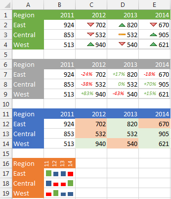
The Sparkline will show an increase or decrease in the data depending on the values of each cell.
How to Show Increase or Decrease in Excel?
Create a Table
A simple way to show an increase or decrease in Excel is to create a table. This can be done by highlighting the data you want to use, then clicking on the “Insert” tab and selecting “Table” from the menu. This will open a dialog box, allowing you to easily customize the table.
You can also use the “Format as Table” feature, which is located under the “Home” tab. This feature allows you to format the table and add formatting options such as color and text effects.
Once you have created the table, you can use the “Calculate” button to add a row or column to the table that shows the difference between the values in the two columns. This will give you a visual representation of the increase or decrease.
Using a Chart
Another way to show an increase or decrease in Excel is to use a chart. This can be done by clicking on the “Insert” tab and selecting “Chart” from the menu. This will open a dialog box, allowing you to choose the type of chart you want to create.
Once you have created the chart, you can customize it by adding labels and data points to the chart. You can also use the “Data Labels” feature, which is located under the “Design” tab, to add labels to the chart. This will allow you to easily identify the difference between the two values.
Formatting the Chart
Once you have created the chart, you can use the “Format” tab to customize the look of the chart. This will allow you to add colors, text effects, and other formatting options to the chart.
You can also use the “Chart Type” feature to choose the type of chart you want to use. This will allow you to choose from a variety of chart types, such as line, bar, and pie charts. This will give you a better visual representation of the increase or decrease.
Using Formulas
You can also use formulas to show an increase or decrease in Excel. This can be done by adding a formula to the cell you want to use and then using the “Calculate” button to calculate the difference between the two values.
For example, if you want to show the difference between two columns of data, you can use the “=” sign and then select the two columns of data you want to use. This will give you a visual representation of the difference between the two values.
Using the IF Function
Another way to show an increase or decrease in Excel is to use the “IF” function. This function can be used to compare two cells and then display the result in a new cell.
For example, you can use the “IF” function to compare two cells and then display the result in a new cell that displays the difference between the two values. This will give you a visual representation of the increase or decrease.
Formatting the Result
Once you have calculated the difference between the two values, you can format the result to make it easier to read. This can be done by using the “Format Cells” feature, which is located under the “Home” tab.
This will allow you to customize the look of the result by adding colors, text effects, and other formatting options. This will make it easier to identify the increase or decrease.
Top 6 Frequently Asked Questions
What are the basic steps for showing increase or decrease in Excel?
The basic steps for showing increase or decrease in Excel are as follows:
1. Enter the data in two columns.
2. Create a clustered column chart.
3. Right-click on the chart and select “Change Series Chart Type”.
4. Select the “Line with Markers” chart type.
5. Add labels to the chart.
6. Select the “Show Trendline” option.
7. Choose the “Linear” trendline type.
8. Select the “Display R-squared Value on Chart” option.
What is a clustered column chart?
A clustered column chart is a type of chart that displays data in two or more columns. It is used to compare two or more sets of data, or to show the trend of a variable over time. The clustered column chart is made up of individual columns that represent each data set, with the length of the column representing the magnitude of the data.
What is the “Line with Markers” chart type?
The “Line with Markers” chart type is a type of chart that combines a line graph with markers. This type of chart is useful for showing trends in data over time, or for comparing data between two or more groups. The line graph shows the trend of the data, while the markers indicate the individual data points.
What is a trendline?
A trendline is a line that is drawn through a set of data points to identify trends in the data. Trendlines can be used to show an overall pattern or trend in the data. For example, if a dataset is showing an increasing trend, the trendline would be drawn in an upward direction.
What is the “Linear” trendline type?
The “Linear” trendline type is a type of trendline that is used to identify linear trends in data. This trendline type fits a straight line to the data points. It is used to identify linear relationships between variables and can be used to predict future values.
What is the “Display R-squared Value on Chart” option?
The “Display R-squared Value on Chart” option is an option that can be selected when creating a trendline in Excel. If this option is selected, the R-squared value for the trendline will be displayed on the chart. The R-squared value is a measure of how closely the trendline is following the data points. A higher R-squared value indicates that the trendline is a better fit for the data.
Knowing how to show increase or decrease in Excel can be an invaluable tool when it comes to analyzing data. By learning the basics, such as how to create sparkline charts, you can quickly and easily visualize data, providing a more comprehensive understanding of the information. With a few simple steps, you can easily create a chart that will effectively demonstrate the increase or decrease in data, allowing anyone to quickly and effectively analyze data.